CIFAR-10 Tutorial
Creating a Neural Network for CIFAR-10 Classification
References:
- The code in this blog post can be found directly from the PyTorch tutorial here.
- For information on the CIFAR-10 dataset, a reference page can be found here.
- In the section marked “Contribution”, the provided code follows directly from the tutorial above, however there were slight modifications made to layer amounts and layer size for the purpose of comparing classification performance.
Goal of this post:
- The goal of this post is to provide an introduction into creating a neural network for classifying the CIFAR-10 data set, and to explore modifications that may or may not improve its accuracy. We will look how these modifications affect the classification performance.
We’ll begin by importing the torch package as we’ll be using some built in functions for building the neural network.
import torch
import torchvision
import torchvision.transforms as transforms
Here, we’re simply downloading and uploading the CIFAR-10 images, while compartmentlizing them to multiple data sets labled “trainset” and “testset”. We’ll also perform an operation called “normalizing” on our datasets. This step is merely for ease of computational performance. We’re not affecting the integrity of the datasets.
# Downloading the CIFAR-10 data set, normalizing the image values in between
# -1 and 1, compartmentalizing the data sets into training and testing sets.
transform = transforms.Compose(
    [transforms.ToTensor(),
     transforms.Normalize((0.5, 0.5, 0.5), (0.5, 0.5, 0.5))])

batch_size = 4

trainset = torchvision.datasets.CIFAR10(root='./data', train=True,
                                        download=True, transform=transform)
trainloader = torch.utils.data.DataLoader(trainset, batch_size=batch_size,
                                          shuffle=True, num_workers=2)

testset = torchvision.datasets.CIFAR10(root='./data', train=False,
                                       download=True, transform=transform)
testloader = torch.utils.data.DataLoader(testset, batch_size=batch_size,
                                         shuffle=False, num_workers=2)

classes = ('plane', 'car', 'bird', 'cat',
           'deer', 'dog', 'frog', 'horse', 'ship', 'truck')
Files already downloaded and verified
Files already downloaded and verified
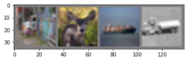
Now, let’s visualize some of the images to see what we’re working with!
import matplotlib.pyplot as plt
import numpy as np

def imshow(img):
    img = img / 2 + 0.5
    npimg = img.numpy()
    plt.imshow(np.transpose(npimg, (1, 2, 0)))
    plt.show()

dataiter = iter(trainloader)
images, labels = dataiter.next()

imshow(torchvision.utils.make_grid(images))
print(' '.join('%5s' % classes[labels[j]] for j in range(batch_size)))
truck deer ship truck
Above, we see some small images of a “horse, frog, dog, and deer”. As a reminder, each image is of size 32x32 pixels.
Building Our Neural Network
At this step, we’ll be creating a simple neural network structure utilzing two convolutional layers and three fully connected layers. We’ll be using the cross-entropy loss function. Our activation functions across each layer will be $f(x) = max{x,0}$.
# Defining our neural network
import torch.nn as nn
import torch.nn.functional as F

class Net(nn.Module):
    def __init__(self):
        super().__init__()
        self.conv1 = nn.Conv2d(3, 6, 5)
        # Maxpool has a kernel size of 2x2 with a stride of 2
        self.pool = nn.MaxPool2d(2, 2)
        self.conv2 = nn.Conv2d(6, 16, 5)
        self.fc1 = nn.Linear(16 * 5 * 5, 120)
        self.fc2 = nn.Linear(120, 84)
        # The last number out has to be the number of classes to predict.
        self.fc3 = nn.Linear(84, 10)

    def forward(self, x):
        x = self.pool(F.relu(self.conv1(x)))
        x = self.pool(F.relu(self.conv2(x)))
        x = torch.flatten(x, 1) # flatten all dimensions except batch
        x = F.relu(self.fc1(x))
        x = F.relu(self.fc2(x))
        x = self.fc3(x)
        return x


net = Net()
# Defining our loss (objective) function and optimizier
import torch.optim as optim

criterion = nn.CrossEntropyLoss()
optimizer = optim.SGD(net.parameters(), lr=0.001, momentum=0.9)
Training Our Neural Network
At this point, we’ve designed our neural network and we’re ready to train our model. We’ll run the network through a series of iterations, hopefully building a decent a prediction function.
for epoch in range(2):  # loop over the dataset multiple times

    running_loss = 0.0
    for i, data in enumerate(trainloader, 0):
        # get the inputs; data is a list of [inputs, labels]
        inputs, labels = data

        # zero the parameter gradients
        optimizer.zero_grad()

        # forward + backward + optimize
        outputs = net(inputs)
        loss = criterion(outputs, labels)
        loss.backward()
        optimizer.step()

        # print statistics
        running_loss += loss.item()
        if i % 2000 == 1999:    # print every 2000 mini-batches
            print('[%d, %5d] loss: %.3f' %
                  (epoch + 1, i + 1, running_loss / 2000))
            running_loss = 0.0

print('Finished Training')
[1,  2000] loss: 2.177
[1,  4000] loss: 1.798
[1,  6000] loss: 1.643
[1,  8000] loss: 1.554
[1, 10000] loss: 1.492
[1, 12000] loss: 1.424
[2,  2000] loss: 1.368
[2,  4000] loss: 1.337
[2,  6000] loss: 1.330
[2,  8000] loss: 1.323
[2, 10000] loss: 1.287
[2, 12000] loss: 1.265
Finished Training
Testing Our Neural Network
Now that we’ve trained our neural network, we can test it on our test data set. Hopefully we’ll get a decent performance!
# Testing our neural network on the test data set
dataiter = iter(testloader)
images, labels = dataiter.next()

# print images
imshow(torchvision.utils.make_grid(images))
print('GroundTruth: ', ' '.join('%5s' % classes[labels[j]] for j in range(4)))


### This part is not necessary ###
net = Net()
net.load_state_dict(torch.load(PATH))
##################################

# Letting the neural network classify the testing data set
outputs = net(images)

# Getting the index of the highest energy
_, predicted = torch.max(outputs, 1)

print('Predicted: ', ' '.join('%5s' % classes[predicted[j]]
                              for j in range(4)))


# Testing to see how the network performs on the whole dataset
correct = 0
total = 0
# since we're not training, we don't need to calculate the gradients for our outputs
with torch.no_grad():
    for data in testloader:
        images, labels = data
        # calculate outputs by running images through the network
        outputs = net(images)
        # the class with the highest energy is what we choose as prediction
        _, predicted = torch.max(outputs.data, 1)
        total += labels.size(0)
        correct += (predicted == labels).sum().item()

print('Accuracy of the network on the 10000 test images: %d %%' % (
    100 * correct / total))
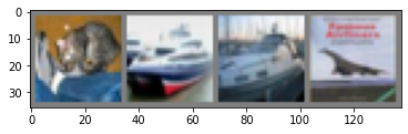
GroundTruth:    cat  ship  ship plane
Predicted:    cat   car   car plane
Accuracy of the network on the 10000 test images: 53 %
# Figuring out what classes performed well vs poorly
# prepare to count predictions for each class
correct_pred = {classname: 0 for classname in classes}
total_pred = {classname: 0 for classname in classes}

# again no gradients needed
with torch.no_grad():
    for data in testloader:
        images, labels = data
        outputs = net(images)
        _, predictions = torch.max(outputs, 1)
        # collect the correct predictions for each class
        for label, prediction in zip(labels, predictions):
            if label == prediction:
                correct_pred[classes[label]] += 1
            total_pred[classes[label]] += 1


# print accuracy for each class
for classname, correct_count in correct_pred.items():
    accuracy = 100 * float(correct_count) / total_pred[classname]
    print("Accuracy for class {:5s} is: {:.1f} %".format(classname,
                                                   accuracy))
Accuracy for class plane is: 65.9 %
Accuracy for class car   is: 83.2 %
Accuracy for class bird  is: 65.4 %
Accuracy for class cat   is: 26.1 %
Accuracy for class deer  is: 30.1 %
Accuracy for class dog   is: 41.3 %
Accuracy for class frog  is: 68.6 %
Accuracy for class horse is: 52.4 %
Accuracy for class ship  is: 58.0 %
Accuracy for class truck is: 48.4 %
Contribution
In this section, we’ll make adjustments to the neural network defined above by increasing the number of network layers and layer size.
Part 1: Changing Neurons Per Layer
In the tutorial, we started with two convolutional layers with given neurons per layer. We’ll vary the number of neurons per layer between 30 and 180. We’ll look at their differences in performances.
# Defining our neural network
information = np.zeros((8,3));
j = 0; N = 200; k = 5; kp = 2;  s = 2;

for n in range(30,181,20):
    learning_rate = 0.0015

    print("Currently training model", j+1, "of 8.")

    class Net(nn.Module):
        def __init__(self):
            super().__init__()

            self.pool = nn.MaxPool2d(kp, s)
            self.conv1 = nn.Conv2d(3, n, k)
            self.conv2 = nn.Conv2d(n, N, k)
            self.fc1 = nn.Linear(N * 5 * 5, 100)
            self.fc2 = nn.Linear(100, 84)
            self.fc3 = nn.Linear(84, 10)

        def forward(self, x):
            x = self.pool(F.relu(self.conv1(x)))
            x = self.pool(F.relu(self.conv2(x)))
            x = torch.flatten(x, 1) # flatten all dimensions except batch
            x = F.relu(self.fc1(x))
            x = F.relu(self.fc2(x))
            x = self.fc3(x)
            return x

    net_multi = Net()
    criterion_multi = nn.CrossEntropyLoss()
    optimizer_multi = optim.SGD(net_multi.parameters(), lr=learning_rate, momentum=0.9)

    # Training our network
    for epoch in range(3):  # loop over the dataset multiple times

        running_loss_multi = 0
        for i, data in enumerate(trainloader, 0):
            inputs, labels = data
            optimizer_multi.zero_grad()
            outputs = net_multi(inputs)
            loss_multi = criterion_multi(outputs, labels)
            loss_multi.backward()
            optimizer_multi.step()

                    # print statistics
            running_loss_multi += loss_multi.item()
            if i % 5000 == 4999:    # print every 5000 mini-batches
                print('[%d, %5d] loss: %.3f' %
                      (epoch + 1, i + 1, running_loss_multi / 5000))
                running_loss_multi = 0.0

    correct = 0
    total = 0

    with torch.no_grad():
        for data in testloader:
            images, labels = data
            # calculate outputs by running images through the network
            outputs = net_multi(images)
            # the class with the highest energy is what we choose as prediction
            _, predicted = torch.max(outputs.data, 1)
            total += labels.size(0)
            correct += (predicted == labels).sum().item()

    information[j,:] = [n,N,100*correct/total]
    j += 1;


print("Finished Training")
Currently training model 1 of 8.
[1,  5000] loss: 1.748
[1, 10000] loss: 1.372
[2,  5000] loss: 1.097
[2, 10000] loss: 1.017
[3,  5000] loss: 0.838
[3, 10000] loss: 0.836
Currently training model 2 of 8.
[1,  5000] loss: 1.734
[1, 10000] loss: 1.328
[2,  5000] loss: 1.071
[2, 10000] loss: 0.997
[3,  5000] loss: 0.821
[3, 10000] loss: 0.811
Currently training model 3 of 8.
[1,  5000] loss: 1.711
[1, 10000] loss: 1.328
[2,  5000] loss: 1.058
[2, 10000] loss: 0.994
[3,  5000] loss: 0.809
[3, 10000] loss: 0.814
Currently training model 4 of 8.
[1,  5000] loss: 1.702
[1, 10000] loss: 1.310
[2,  5000] loss: 1.033
[2, 10000] loss: 0.959
[3,  5000] loss: 0.782
[3, 10000] loss: 0.784
Currently training model 5 of 8.
[1,  5000] loss: 1.703
[1, 10000] loss: 1.332
[2,  5000] loss: 1.050
[2, 10000] loss: 0.968
[3,  5000] loss: 0.799
[3, 10000] loss: 0.795
Currently training model 6 of 8.
[1,  5000] loss: 1.707
[1, 10000] loss: 1.318
[2,  5000] loss: 1.061
[2, 10000] loss: 0.973
[3,  5000] loss: 0.801
[3, 10000] loss: 0.800
Currently training model 7 of 8.
[1,  5000] loss: 1.695
[1, 10000] loss: 1.311
[2,  5000] loss: 1.040
[2, 10000] loss: 0.964
[3,  5000] loss: 0.790
[3, 10000] loss: 0.789
Currently training model 8 of 8.
[1,  5000] loss: 1.707
[1, 10000] loss: 1.303
[2,  5000] loss: 1.029
[2, 10000] loss: 0.967
[3,  5000] loss: 0.784
[3, 10000] loss: 0.797
Finished Training
plt.bar(information[:,0], information[:,2], width = 10)
plt.xlabel("Number of Neurons Per Hidden Layer")
plt.ylabel("% Accuracy")
plt.title("% Accuracy vs Neurons Per Hidden Layer")
print(information)
[[ 30.   200.    70.73]
 [ 50.   200.    71.15]
 [ 70.   200.    67.49]
 [ 90.   200.    71.42]
 [110.   200.    71.  ]
 [130.   200.    70.44]
 [150.   200.    70.49]
 [170.   200.    70.61]]
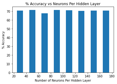
The table above displays the different number of neurons in the input and output layer, respectively, followed by the percent accuracy of prediction. The best prediction accuracy was 71.42% when 90/200 neurons were used. The worst prediction accuracy was 67.49% when 50/200 neurons were used. We’d like to note that the prediction accuracy of each test was better than the tutorial prediction of 53%. The bar-chart displays the same information as the table above.
Part 2: Changing Layer Amounts
In this section, we’ll change the number of convolutional layers to 3 and 4. We’ll take the best performing model above and have similar neuron amounts per layer. Similarly, we’ll look at the differences in performances.
2.1) 3 Convolutional Layers - 3 Fully Connected Layers
For our first variation, we’ll add an additional convoluted layer for a total of three convolutional layers coupled with three fully connected layers. We’d like to note that in the previous section, the differences in the prediction accuracies based off of the neurons per hidden layer were small, so in this section we’ll utilize roughly the same amount of neurons per hidden layer, while keeping the filter size as a $5 \times 5$.
N = 240; k=5;
learning_rate = 0.002;

class Net(nn.Module):
    def __init__(self):
        super().__init__()

        # Maxpool has a kernel size of 2x2 with a stride of 2.
        self.pool = nn.MaxPool2d(kp, s)

        # Defining our convolutional layers.
        self.conv1 = nn.Conv2d(3, 100, k)
        self.conv2 = nn.Conv2d(100, 180, k)
        self.conv3 = nn.Conv2d(180, N, k)
        self.fc1 = nn.Linear(N * 1 * 1, 100)
        self.fc2 = nn.Linear(100, 200)
        self.fc3 = nn.Linear(200, 10)

    def forward(self, x):
        x = self.pool(F.relu(self.conv1(x)))
        x = self.pool(F.relu(self.conv2(x)))
        x = F.relu(self.conv3(x))
        x = torch.flatten(x, 1) # flatten all dimensions except batch
        x = F.relu(self.fc1(x))
        x = F.relu(self.fc2(x))
        x = self.fc3(x)
        return x

net_2 = Net()
criterion_2 = nn.CrossEntropyLoss()
optimizer_2 = optim.SGD(net_2.parameters(), lr=learning_rate, momentum=0.9)

# Training our network
for epoch in range(4):  # loop over the dataset multiple times

    loss_ph1 = 0; loss_ph2 = 0;
    running_loss_2 = 0
    for i, data in enumerate(trainloader, 0):
        inputs, labels = data
        optimizer_2.zero_grad()
        outputs = net_2(inputs)
        loss_2 = criterion_2(outputs, labels)
        loss_2.backward()
        optimizer_2.step()

        # print statistics
        running_loss_2 += loss_2.item()
        if i % 2000 == 1999:    # print every 2000 mini-batches
            print('[%d, %5d] loss: %.3f' %
                  (epoch + 1, i + 1, running_loss_2 / 2000))
            running_loss_2 = 0.0
        loss_ph2 = loss_ph1;
        loss_ph1 = 0;

correct = 0
total = 0

with torch.no_grad():
    for data in testloader:
        images, labels = data
        outputs = net_2(images)
        _, predicted = torch.max(outputs.data, 1)
        total += labels.size(0)
        correct += (predicted == labels).sum().item()

print("We predicted ", 100*correct/total, "% correct using 3 Convolutional Layers and 3 Fully Connected Layers")
[1,  2000] loss: 2.339
[1,  4000] loss: 1.648
[1,  6000] loss: 1.496
[1,  8000] loss: 1.398
[1, 10000] loss: 1.317
[1, 12000] loss: 1.227
[2,  2000] loss: 1.440
[2,  4000] loss: 1.072
[2,  6000] loss: 1.029
[2,  8000] loss: 1.010
[2, 10000] loss: 0.973
[2, 12000] loss: 0.986
[3,  2000] loss: 1.040
[3,  4000] loss: 0.841
[3,  6000] loss: 0.827
[3,  8000] loss: 0.798
[3, 10000] loss: 0.800
[3, 12000] loss: 0.802
[4,  2000] loss: 0.830
[4,  4000] loss: 0.651
[4,  6000] loss: 0.667
[4,  8000] loss: 0.648
[4, 10000] loss: 0.662
[4, 12000] loss: 0.680
We predicted  70.49 % correct using 3 Convolutional Layers and 3 Fully Connected Layers
The prediction accuracy of our model was 70.49% which is similar to the prediction accuracies from the previous section. In the next section, we’ll add a fourth convolutional layer and explore the differences in performance.
2.1) 4 Convolutional Layers - 3 Fully Connected Layers
In this section, we’ll add a fourth convolutional layer to our model for a total of four convolutional layers and three fully connected layers. In addition, we’ll change the filter size in the last two convolutional layers from $5 \times 5$’s to $2 \times 2$’s. The neurons per hidden convolutional layer are similar to the previous sections.
import torch.nn as nn
import torch.nn.functional as F
import torch.optim as optim

N = 300; k=3; kp = 2; s = 2;
learning_rate = 0.005

class Net(nn.Module):
    def __init__(self):
        super().__init__()

        self.pool = nn.MaxPool2d(kp, s)
        self.conv1 = nn.Conv2d(3, 100, k)
        self.conv2 = nn.Conv2d(100, 180, k)
        self.conv3 = nn.Conv2d(180, 240, 2)
        self.conv4 = nn.Conv2d(240, N, 2)
        self.fc1 = nn.Linear(N * 1 * 1, 100)
        self.fc2 = nn.Linear(100, 200)
        self.fc3 = nn.Linear(200, 10)

    def forward(self, x):
        x = self.pool(F.relu(self.conv1(x)))
        x = self.pool(F.relu(self.conv2(x)))
        x = self.pool(F.relu(self.conv3(x)))
        x = F.relu(self.conv4(x))
        x = torch.flatten(x, 1) # flatten all dimensions except batch
        x = F.relu(self.fc1(x))
        x = F.relu(self.fc2(x))
        x = self.fc3(x)
        return x

net_3 = Net()
criterion_3 = nn.CrossEntropyLoss()
optimizer_3 = optim.SGD(net_3.parameters(), lr=learning_rate, momentum=0.9)

# Training our network
for epoch in range(4):  # loop over the dataset multiple times

    loss_ph1_2 = 0; loss_ph2_2 = 0;
    running_loss_3 = 0
    for i, data in enumerate(trainloader, 0):
        # get the inputs; data is a list of [inputs, labels]
        inputs, labels = data

        # zero the parameter gradients
        optimizer_3.zero_grad()

        # forward + backward + optimize
        outputs = net_3(inputs)
        loss_3 = criterion_3(outputs, labels)
        loss_3.backward()
        optimizer_3.step()

        # print statistics
        running_loss_3 += loss_3.item()
        if i % 1000 == 999:    # print every 1000 mini-batches
            print('[%d, %5d] loss: %.3f' %
                  (epoch + 1, i + 1, running_loss_3 / 1000))
            running_loss_3 = 0.0

correct = 0
total = 0

    # since we're not training, we don't need to calculate the gradients for our outputs
with torch.no_grad():
    for data in testloader:
        images, labels = data
        # calculate outputs by running images through the network
        outputs = net_3(images)
        # the class with the highest energy is what we choose as prediction
        _, predicted = torch.max(outputs.data, 1)
        total += labels.size(0)
        correct += (predicted == labels).sum().item()

print("We predicted", 100*correct/total, "% correct using 4 Convolutional Layers and 3 Fully Connected Layers")
[1,  1000] loss: 2.257
[1,  2000] loss: 2.049
[1,  3000] loss: 1.942
[1,  4000] loss: 1.801
[1,  5000] loss: 1.733
[1,  6000] loss: 1.681
[1,  7000] loss: 1.627
[1,  8000] loss: 1.538
[1,  9000] loss: 1.551
[1, 10000] loss: 1.488
[1, 11000] loss: 1.455
[1, 12000] loss: 1.491
[2,  1000] loss: 1.386
[2,  2000] loss: 1.359
[2,  3000] loss: 1.356
[2,  4000] loss: 1.357
[2,  5000] loss: 1.311
[2,  6000] loss: 1.291
[2,  7000] loss: 1.291
[2,  8000] loss: 1.280
[2,  9000] loss: 1.305
[2, 10000] loss: 1.281
[2, 11000] loss: 1.265
[2, 12000] loss: 1.256
[3,  1000] loss: 1.167
[3,  2000] loss: 1.149
[3,  3000] loss: 1.160
[3,  4000] loss: 1.148
[3,  5000] loss: 1.187
[3,  6000] loss: 1.161
[3,  7000] loss: 1.165
[3,  8000] loss: 1.175
[3,  9000] loss: 1.154
[3, 10000] loss: 1.136
[3, 11000] loss: 1.133
[3, 12000] loss: 1.129
[4,  1000] loss: 1.038
[4,  2000] loss: 1.043
[4,  3000] loss: 1.055
[4,  4000] loss: 1.111
[4,  5000] loss: 1.075
[4,  6000] loss: 1.058
[4,  7000] loss: 1.091
[4,  8000] loss: 1.097
[4,  9000] loss: 1.122
[4, 10000] loss: 1.138
[4, 11000] loss: 1.100
[4, 12000] loss: 1.105
We predicted 61.33 % correct using 4 Convolutional Layers and 3 Fully Connected Layers
In this section, we’ll add a fourth convolutional layer to our model for a total of four convolutional layers and three fully connected layers. In addition, we’ll change the filter size in the last two convolutional layers from $5 \times 5$’s to $2 \times 2$’s. The neurons per hidden convolutional layer are similar to the previous sections.
Conclusion
The tutorial used throughout this post was a wonderful stepping stone for understanding the basic uses and framework of convolutional neural networks. As we experimented with different variations of the original model, we had our best performance of 71.42% which was realized with two convolutional layers and two fully connected layers. The next step would be to explore a larger scale of neurons per layer as well as different activation functions besides $f(x) = max{x,0}$.